Machine Learning Summary
from the Stanford AI Class video sets #5&6
Michael Schippling
-- Oct 27, 2011
Machine Learning extracts information from raw data
Introduction and Terminology
Bayes Network Classifiers
Linear Regression
Clustering
Perceptrons
K Nearest Neighbor
K-Means
Expectation Maximization and Gaussians
Introduction and Terminology
Machine Learning uses a Training
Set of example inputs and attempts to build a model which
will
predict the output when given a new Input.
Why?
- Prediction
- Diagnostics
- Summarization
What it looks for
- Parameters
-- e.g. the nodes of a Bayes Network or the coefficients of a
descriptive equation;
- Structure
-- e.g. the arcs of a Bayes Network;
- Hidden
concepts -- e.g. finding clusters of data which form
groups;
How it interacts
- Passive
-- as an observer only;
- Active
-- has effect on its environment;
- Online
-- while data is being generated;
- Offline
-- after data is generated;
What it does
- Classification
-- put data into a discrete number of classes, often binary;
- Regression
-- continuous prediction, e.g. given today's temperature what will it
be tomorrow?
Types
- Supervised
-- the Input Training Set contains associated Target Labels, i.e.
result values;
- Un-supervised -- the Training Set does NOT
contain Target Labels;
- Reinforcement -- the environment supplies
feedback, effectively combining the Training Set and Targets;
Models
The object of Machine Learning is to build a useful model. If the model
is too specific it will Overfit
-- it will be too specific to the Training Data and may not work
correctly with new data. If the model is not specific enough it will Underfit and fail
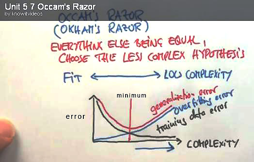
to work well on the Training Data. There is a trade off between the
complexity of the model and its error rate which needs to be minimized.
Here the red curve shows the trade off :
Data Sets
The Training Set is (usually) a large list of data vectors or sets
of values:
{X1, X2, ... Xn}
each of which represent a condition of the system under consideration.
In
Supervised Learning these vectors will be accompanied by a
result or Target Label value:
{X1, X2, ... Xn}
-> Y
where Y may be a classification, e.g. Black or White, or a continuous
value, e.g. 98.6 degrees.
In order to build and test a model the full data set can be divided
into three sub-sets using these approximate percentages:
Training -- 80% --
Used for the actual model building;
Cross-validation
-- 10% -- Used to test the complexity of the trained model,
i.e., how overfitted is it?
Test -- 10%
-- Used for the final model validation.
The Training and Cross-validation sets can be mixed and
re-divided in order to do multiple training runs using different
model-building parameters, but the Test set should be independent in
order to minimize final errors.
Bayes Network Classifiers
A Classifier tries to put data into classes that have common
attributes. A simple example would be to decide if an image pixel was
Black or White. The Video lesson presented the example of deciding if
an email message was Spam or Ham... To do this we take a set of
messages which have already been correctly classified and then look at
the frequency of word use in each set -- under the assumption that Spam
uses words differently than real messages. This is called Bag of Words.
Maximum Likelihood
The initial approach is to determine the probability of each word
(W) occurring in the two sets, Spam and notSpam (S, ~S) and then
calculate the probability that the words in a new message (M) are in
either set. To do this:
- Calculate P(S) and P(~S), the probability of S and ~S
messages: messages-in-the-set / total-number-of-messages;
- Find the unique set of words used in the full input corpus:
this makes a dictionary
or a set of word classes
to count;
- Count the use of each word in each message
set: how many times is the word used in S and ~S?
- Calculate P(Wn|S), the probability
that each word is in
each set: words-in-the-set / total-words-in-the-set;
- Do the Bayesian thing to calculate whether a message is
Spam
or not: P(S|M) = P(W1|S) * P(W2|S)
* P(S) / P(M)
Laplace Smoothing with K=N
With the naive Maximum Likelihood model we quickly find that there is
overfitting due to under-sampling of some words in the corpus: if a
word doesn't appear in the Spam category it will automatically prevent
any message containing that word from being classified as Spam. A
solution is to add a constant value, K, to the count of each
word in each set, and then re-calculate their probabilities. This is
called Laplace Smoothing with K=N (note that this adds K to every
message and word count). The example adds K=1 to every class and set in
the model, and has the effect of less-horribly miss-classifying low
probability messages. It Smooths
Out the distributions.
Example
A spreadsheet for the Spam example (videos 5.7-5.17) can be viewed in your browser here, or
get the original here.
Linear Regression
Regression attempts to find a function that will model a data set
that has continuous values. A non-simple example would take the input
vector X:
{todays-temperature, todays-humidity, TulsaOK-temperature,
big-toe-pain} and try to predict the Target Y:
{tomorrows-rainfall}. Regression functions are generally polynomials
and the job of the Machine Learner is to estimate the W parameters so as
to minimize the errors in the model:
Yi = W0 + W1*Xi
+ W2*Xi2
+ ...
Note that W and X are vectors of values, where the number of values
is the dimension
of the system, and the * operations are vector cross-products. The
degree of
the polynomial is the maximum power to which X is taken. Fortunately,
for this class, we only deal with single dimension variables --
good'ole numbers -- and degree 1 or Linear polynomials
-- good'ole straight lines -- so the functions we want have this form:
Yi
= W0 + W1*Xi
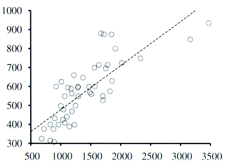
What we are trying to do is draw a line through the data set that
minimizes the total distance between the line and each data point, as
shown here:
where W0 is the Y
Intercept (where our line crosses the vertical axis at X=0) and
W1 is the Slope.
It turns out to be "easy" to do (modulo a lot of algebra and derivative
taking) using a Quadratic
Loss
equation that minimizes the squared error over all the input points.
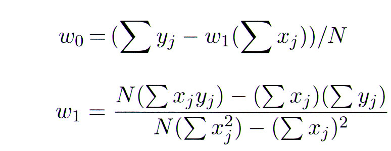
Given a data set of x,y pairs, the optimal Linear Regression W
parameters can be calculated with these equations -- where Xj and Yj
are each x,y pair in the data set and N is the number of pairs:
Example
A spreadsheet for the video 5.24 example can be viewed in your browser here,
or
get the original here.
Problems with Linear Regression
- Straight lines don't fit curves very well;
- Outliers in the data skew the regression
- As you go to infinity on X, so does Y, which may not make
sense for your model.
e.g. the weather may not be getting hotter and hotter;
Some
of these problems can be addressed with Smoothing algorithms, such as a
Logistic Function
or Regularization
which tend to pull the parameter
values away from extremes. But once these functions become more
complicated they don't have closed form solutions and have to be solved
iteratively -- by trying different values to see how well they work.
One method for this is Gradient
Descent -- a search down a slope for a
minimum. This can have problems with finding local solutions rather
than the global minimum, but sometimes that's better than nothing.
Clustering
Clustering is a way of classifying continuous data points into sub-sets
that are "near" each other, or have similar attributes.
The simplest version is Linear
Separation -- drawing a line between two groups. If the
data points are already labeled with their class, i.e., Supervised
Learning with the outputs specified, this can be as "easy" as finding a
line that lies between the two groups, assuming that the groups are
Linearly Separable -- they are not mixed together in the input space --
to start with. If the data is not labeled then it
is Un-Supervised Learning, and the job is to find a separator
based on how close each group's points are to each other -- assigning
data points to particular groups in the process.
The divisions between clusters are called Voroni Graphs or Fronts.
There are many clustering algorithms. A few are outlined
below.
Perceptrons
A Perceptron
is a simple model of a biological neuron. It updates its
internal parameter weights
in an iterative cycle to reduce the errors in its output using Gradient
Descent to find a minimum. For the case of a Linear
Separator, the parameters are the W0 and W1 coefficients of the line
equation -- just as for Linear Regression. The Perceptron update rule
also uses the same technique as regression to find minima, it subtracts a bit of the error from the parameter and tries again:
Wi
= Wi + a
* (y - f(x))
Wi is the parameter of interest and (y -
f(x)) is the difference
between a data point's actual Y value and the value "predicted" by the
function f(x) using the current Wi value, i.e.,
the error in the
prediction. a
-- alpha
-- is a small Learning
Rate
coefficient, often in the range of .001, which controls how much of the
error feeds-back into Wi on each update cycle.
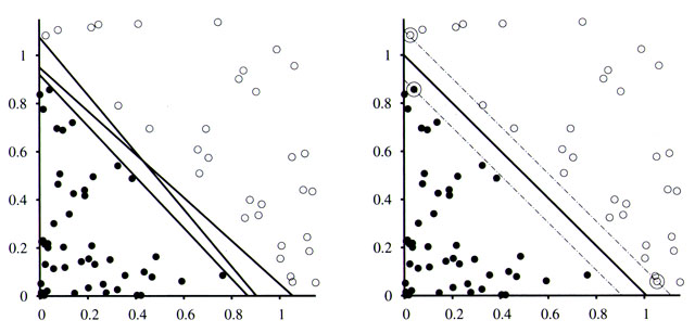
A Perceptron is guaranteed to converge to a Linear Separator, if one
exists. However, it can find one of many possible separators and may
not find the optimal one. To improve on this we want to maximize the margin -- distance
-- between the separator and the data points, as shown on the left in
the Clustering image. One way to do this is with a Support Vector Machine (SVM)
which uses a Quadratic
Programming optimization to generalize the error
calculations. Using the Kernel Trick an SVM can also modify its internal model to use
higher order polynomials and thus find non-linear cluster
separators, e.g., circles.
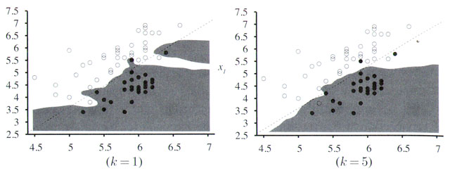
K Nearest Neighbor
The KNN
algorithm does pretty much what it says: For a new data point, find the
number=K neighbors which are closest in the input space and use them to
classify the new point. For K=1 this is just finding the nearest
classified point and using it's value. For K>1 you find that many
neighbors and average their values.
When
building the models one can use cross-validation to find a good K
because there's a tradeoff between the complexity of the data and the
goodness of the fit. Using a large K gives a smoother result but may
mis-classify outliers. There are also problems searching in large data
sets, but these can be fixed with tree or hash data structures. There
are worse problems with high dimensional data because it is
exponentially more likely that a point will be very distant from others.
K-Means
The K-Means algorithm is an un-supervised clustering
tool. The K parameter is the number of clusters to find, for instance
K=2 will find two clusters that may not have a Linear Separator. It
will converge to a locally optimal clustering, perhaps after a few
iterations. In general clustering is NPhard so a locally optimal
solution is pretty good.
The algorithm is:
- Start by guessing number=K cluster centers at random;
- For each center find their set of most likely data points by Euclidean distance.
Each center separates the space and the line between is the "equidistant line"; - Find the two points that are at the geometric center of these preliminary clusters;
- Move the centers to those points;
- Iterate from 2 -- re-assign points to the centers and then re-center until the centers don't move anymore;
- If a cluster center becomes empty -- has no data points associated -- then restart with new random selections.
The problems with this are:
- Need to know K, i.e., How many clusters are we looking for?
- It finds a local minimum;
- Same general problem with high dimensionality as KNN;
- There's no mathematical basis -- it only works in practice...
Expectation Maximization and Gaussians
We can use Gaussian distributions in place of straight-ahead Euclidean
distances when calculating KNN or K-Means separations. This effectively
puts non-linearly decreasing probability "fields" around each point,
and then we can use the posterior probabilities of all the points
combined to decide which centers to associate with. In this case data
points are never completely "cut-off" from any center, but some centers
have a higher probability of association than others. This smooths the
transitions of the centers during the iterated search and also reduces
the effect of outlier data points on the results.
Using
Gaussians with the K-Means algorithm is called Expectation Maximization
and the two algorithms may converge to different data models.
